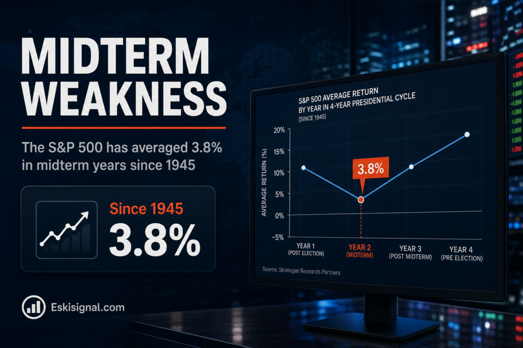
Americans vote on 3 November. The statistic that will be quoted at every point between now and then is that since 1945 the S&P 500 has averaged 3.8% in midterm years against 10.9% in the other three years of the presidential cycle. It is a real number, accurately calculated, and it is built on twenty observations. Both halves of that sentence matter.
This article is for informational and educational purposes only. It is not financial advice, investment advice, or a recommendation to buy, sell, or hold any security, cryptocurrency, or financial product. Always verify data with official sources before making financial decisions.
Short answer: weakest year, strongest aftermath, tiny sample
Short answer: The historical pattern has three parts. Midterm years have been the weakest of the four-year cycle, averaging 3.8% since 1945. Volatility has typically been elevated from spring into autumn. And the aftermath has been unusually strong — since 1974 the index has averaged 5.7% in the three months following a midterm, positive in 11 of 13 instances, and roughly 12.4% over the following twelve months. The pattern is consistent enough to be interesting and the sample is small enough that it should not be traded mechanically.
The mechanism people propose, and whether it holds up
The standard explanation is uncertainty resolution. Markets dislike unresolved policy risk, midterms create a period where the direction of tax, spending and regulatory policy is genuinely unknown, and the removal of that uncertainty on election night releases a risk premium regardless of who wins.
The evidence for this is better than the evidence for most seasonal stories, because the effect is not symmetric around the outcome. If the pattern were about policy preference, results should differ substantially depending on which party gained control. They largely do not. What appears to matter is that the question is settled, not how it is settled — which is what an uncertainty premium looks like and is not what a policy-preference effect looks like.
A second, less flattering mechanism is worth stating alongside it. Divided government tends to follow midterms, and divided government produces legislative gridlock. Equity markets have historically been comfortable with gridlock, because the range of possible policy outcomes narrows sharply. That is not a claim about good governance. It is a claim about variance.
| Period | S&P 500 average | Observations |
|---|---|---|
| Midterm years, 1945-2025 | +3.8% | 20 |
| Other three years of cycle | +10.9% | 60 |
| Three months after midterm, since 1974 | +5.7%, positive 11 of 13 | 13 |
| Twelve months after midterm | ~+12.4% | 13 |
Why twenty observations is the real story
Eighty years of data sounds substantial until the unit of observation is counted. There have been twenty midterm years since 1945 and thirteen usable post-election windows in the shorter series. A single outlier — 2008, say, or 1974 — moves a twenty-observation average by a great deal.
The distribution matters more than the mean here, and it is rarely published alongside it. An average of 3.8% built from a wide spread of individual years tells you something quite different from the same average built from years clustered around it. Any presentation of this statistic that does not show the range of outcomes is presenting the least informative summary of the data available.
There is also a confounding problem that is hard to escape. Midterm years are not randomly assigned; they arrive on a fixed schedule that has, over this sample, repeatedly coincided with particular phases of monetary policy cycles and with recessions that had nothing to do with elections. Separating a calendar effect from the business cycle with twenty data points is not something the data supports, whatever the tidiness of the averages suggests.
What is different about this particular midterm year
Seasonal patterns describe the residual after the large forces are accounted for. This year the large forces are unusually large.
Crude oil is above $100 on an unresolved conflict. The Federal Reserve is being priced for a rate increase rather than a cut, and the White House is publicly lobbying against it. Diesel refining margins set an all-time record last month. Any one of these would ordinarily dominate a calendar effect worth a few percentage points, and there are several of them operating simultaneously.
The reasonable use of the seasonal statistic is therefore as context rather than as a forecast: it establishes that autumn weakness in a midterm year is unremarkable, which is useful mainly as a guard against over-interpreting an ordinary drawdown as the start of something structural. The institutions that publish this research say much the same thing in their own caveats — that growth, inflation, rates and earnings drive returns far more consistently than the electoral calendar does.
The honest counterargument
The strongest case against the whole framework is that it is a well-documented pattern in a market that reads its own research.
Every major asset manager publishes a midterm-cycle note. If the post-election rally were a reliable, exploitable feature of the calendar, positioning would move ahead of it and the effect would erode — which is the ordinary fate of published seasonal anomalies once they are widely known. The counter is that most participants cannot act on a three-month horizon effect of this size after costs, which is why some seasonal patterns persist despite being public. That is a plausible argument and not a proven one.
What this article does not conclude
Nothing here forecasts the election, the market’s reaction to it, or returns over any horizon. Historical averages are descriptions of a small sample of the past and carry no information about any individual future year.
Figures cited are drawn from published research by major asset managers and banks, which differ from one another depending on start date, index used, whether returns are total or price-only, and how the post-election window is defined. Two houses can publish different numbers for the same phenomenon without either being wrong, and comparing across them requires reading the methodology footnote rather than the headline.